|
The objective of this problem is the discovery of a symbolic expression that satisfies a set of fitness cases. Consider we are given a sampling of the numerical values from the function:
|
y = a4 +
a3 + a2 + a |
(6.1) |
over 10 chosen points and we want to find a function fitting those values within 0.01 of the correct value.
First, the set of functions F and the set of terminals T must be chosen. In this case
F = {+, -, *, /} and T = {a}. Then the structural organization of chromosomes, namely the length of the head and the number of genes, is chosen. It is advisable to start with short, single-gene chromosomes and then gradually increase
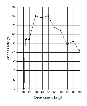
h. Figure 6 shows such an analysis for this problem. A population size
P of 30 individuals and an evolutionary time G of 50 generations were used. A
pm equivalent to two one-point mutations per chromosome and a
p1r = 0.7 were used in all the experiments in order to simplify the analysis. The set of fitness cases is shown in
Table 1 and the fitness was evaluated by equation
(4.1a), being M = 100. If |C(i,j)-Tj| is equal to or less than 0.01 (the precision), then |C(i,j)-Tj|
= 0 and f(i,j) = 100; thus for Ct = 10,
fmax = 1000.

Figure 6. Variation of success rate (Ps) with chromosome length. For this analysis
G = 50, P = 30, and Ps was evaluated over 100 identical runs.
Table 1
Set of fitness cases for the symbolic regression problem.
| a |
f(a) |
| 2.81 |
95.2425 |
| 6 |
1554 |
| 7.043 |
2866.5486 |
| 8 |
4680 |
| 10 |
11110 |
| 11.38 |
18386.0341 |
| 12 |
22620 |
| 14 |
41370 |
| 15 |
54240 |
| 20 |
168420 |
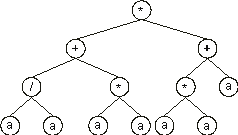
Note that GEP can be useful in searching the most parsimonious solution to a problem. For instance, the chromosome:
0123456789012
*++/**aaaaaaa
with h = 6 codes for the ET:

which is equivalent to the target function (6.1). Note also that GEP can efficiently evolve solutions using large values of
h, that is, it is capable of evolving large and complex sub-ETs. It is worth noting that the most compact genomes are not the most efficient. Therefore a certain redundancy is fundamental to efficiently evolve good programs.
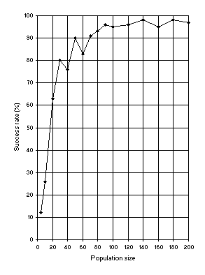
In another analysis, the relationship between success rate and population size
P, using an h = 24 was studied (Figure
7). These results show the supremacy of a genotype/phenotype representation, as this single-gene system, which is equivalent to GP, greatly surpasses that technique
[9]. However, GEP is much more complex than a single-gene system because GEP chromosomes can encode more than one gene (see
Figure 8).

Figure 7. Variation of success rate (Ps) with population size. For this analysis
G = 50, and a medium value of 49 for chromosome length (h = 24) was used.
Ps was evaluated over 100 identical runs.
Suppose we could not find a solution after the analysis shown in Figure
6. Then we could increase the number of genes, and choose a function to link them. For instance, we could choose an
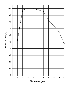
h = 6 and then increase the number of genes gradually. Figure 8 shows how the success rate for this problem depends on the number of genes. In this analysis, the
pm was equivalent to two one-point mutations per chromosome,
p1r = 0.2, p2r = 0.5, pgr = 0.1,
pis = 0.1, pris = 0.1, pgt = 0.1, and three transposons (both IS and RIS elements) of lengths 1, 2, and 3 were used. Note that GEP can cope very well with an excess of genes: the success rate for the 10-genic system is still very high (47%).

Figure 8. Variation of success rate (Ps) with the number of genes. For this analysis
G = 50, P = 30, and h = 6 (a gene length of 13).
Ps was evaluated over 100 identical runs.
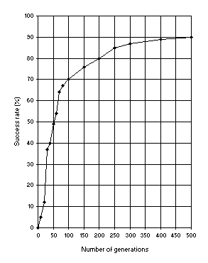
In Figure 9 another important relationship is shown: how the success rate depends on evolutionary time. In contrast to GP where 51 generations are the norm, for after that nothing much can possibly be discovered
[7], in GEP, populations can adapt and evolve indefinitely because new material is constantly being introduced into the genetic pool.

Figure 9. Variation of success rate (Ps) with the number of
generations. For this analysis P = 30, pm = 0.051,
p1r = 0.7 and a chromosome length of 79 (a single-gene chromosome with
h = 39) was used. Ps was evaluated over 100 identical runs.
Finally, suppose that the multigenic system with sub-ETs linked by addition could not evolve a satisfactory solution. Then we could choose another linking function, for instance, multiplication. This process is repeated until a good solution has been found.
As stated previously, GEP chromosomes can be easily modified in order to encode the linking function as well. In this case, for each problem the ideal linking function would be found in the process of adaptation.
Consider, for instance, a multigenic system composed of 3 genes linked by addition. As shown in
Figure 8, the success rate has in this case the maximum value of 100%.
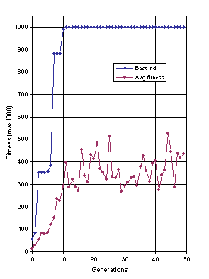
Figure 10 shows the progression of average fitness of the population and the fitness of the best individual for run 0 of the experiment summarized in
Table 2, column 1.

Figure 10. Progression of average fitness of the population and the fitness of the best individual for run 0 of the experiment summarized in
Table 2, column 1 (symbolic regression).
In this run, a correct solution was found in generation 11 (the sub-ETs are linked by
addition):
012345678901201234567890120123456789012
**-*a+aaaaaaa++**a*aaaaaaa*+-a/aaaaaaaa
and mathematically corresponds to the target function (the contribution of each sub-ET is indicated in brackets):
y = (a4) + (a3 + a2 +
a) + (0) = a4 + a3 + a2 +
a.
The detailed analysis of this program shows that some of the actions are redundant for the problem at hand, like the addition of 0 or multiplication by 1. However, the existence of these unnecessary clusters, or even pseudogenes like gene 3, is important to the evolution of more fit individuals (compare, in Figures
6 and 8, the success rate of a compact, single-gene system with
h = 6 with other less compact systems both with more genes and
h greater than 6).
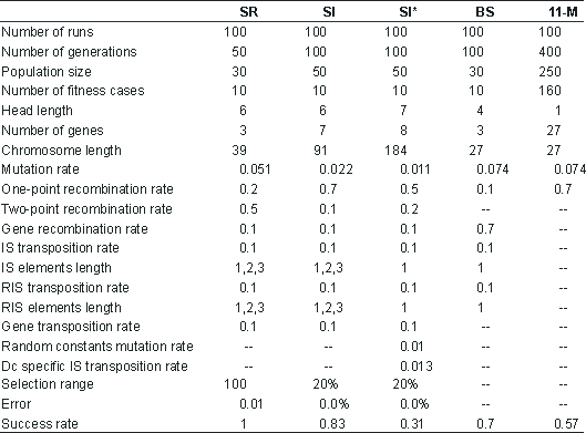
Table 2
Parameters for the symbolic regression (SR), sequence induction (SI), sequence induction using ephemeral random constants (SI*), block stacking (BS), and 11-multiplexer (11-M) problems.

The plot for average fitness in Figure 10 (and also Figures
12, 13 and 17 below) suggests different evolutionary dynamics for GEP populations. The oscillations on average fitness, even after the discovery of a perfect solution, are unique to GEP. A certain degree of oscillation is due to the small population sizes used to solve the problems presented in this work. However, an identical pattern is obtained using larger population sizes.
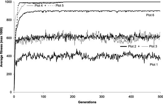
Figure 11 compares six evolutionary dynamics in populations of 500 individuals for 500 generations. Plot 1 (all operators active) shows the progression of average fitness of an experiment identical to the one summarized in
Table 2, column 1, that is, with all the genetic operators switched on. The remaining dynamics were obtained for mutation alone (Plot 2), for gene recombination combined with gene transposition (Plot 3), for one-point recombination (Plot 4), two-point recombination (Plot 5), and gene recombination (Plot 6).

Figure 11. Possible evolutionary dynamics for GEP populations. For this analysis
P = 500. The plots show the progression of average fitness of the population.
Plot 1: All operators switched on with rates as shown in Table
2, column 1; in this case a perfect solution was found in generation 1.
Plot 2: Only mutation at pm = 0.051; in this case a perfect solution was found in generation 3.
Plot 3: Only gene recombination at pgr = 0.7 plus gene transposition at
pgt = 0.2 were switched on; in this case a perfect solution was found in generation 2.
Plot 4: Only one-point recombination at p1r = 0.7; in this case a perfect solution was found in generation 3.
Plot 5: Only two-point recombination at p2r = 0.7; in this case a perfect solution was found in generation 1.
Plot 6: Only gene recombination at pgr = 0.7; in this case a perfect solution was not found: the best of run has fitness 980 and was found in generation 2.
It is worth noticing the homogenizing effect of all kinds of recombination. Interestingly, this kind of pattern is similar to the evolutionary dynamics of GAs and GP populations
[9, 10]. Also worth noticing is the plot for gene recombination alone
(Figure 11, Plot 6): in this case a perfect solution was not found. This shows that sometimes it is impossible to find a perfect solution only by shuffling existing building blocks, as is done in all GP implementations without mutation. Indeed, GEP gene recombination is similar in effect to GP recombination, for it permits exclusively the recombination of mathematically concise blocks. Note that even a more generalized shuffling of building blocks (using gene recombination combined with gene transposition) results in oscillatory dynamics
(Figure 11, Plot 3).
|
