The problem of sequence induction is a special case of symbolic regression where the domain of the independent variable consists of the nonnegative integers. However, the sequence chosen is more complicated than the expression used in symbolic regression, as different coefficients were used.

The solution to this kind of problem involves the discovery of certain constants. Here two different approaches to the problem of constant creation are shown: one without using ephemeral random constants [9], and another using ephemeral random constants.

In the sequence 1, 15, 129, 547, 1593, 3711, 7465, 13539, 22737, 35983, 54321,..., the nth (N) term is:

(6.2)

where a_n consists of the nonnegative integers 0, 1, 2, 3,....

For this problem F = {+, -, *, /} and T = {a}. The set of fitness cases is shown in Table 3 and the fitness was evaluated by equation (4.1b), being M = 20%. Thus, if the 10 fitness cases were computed exactly, f_max = 200.

Table 3
Set of fitness cases for the sequence induction problem.

a	N
1	15
2	129
3	547
4	1593
5	3711
6	7465
7	13539
8	22737
9	35983
10	54321

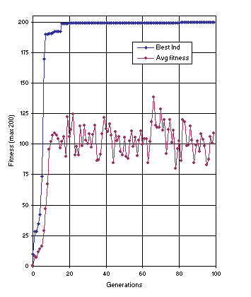
Figure 12 shows the progression of average fitness of the population and the fitness of the best individual for run 1 of the experiment summarized in Table 2, column 2. In this run, a perfect solution was found in generation 81 (the sub-ETs are linked by addition):

0123456789012012345678901201234567890120123456789012012345678901201234567890120123456789012
*a/+a*aaaaaaa**-/**aaaaaaa**+++*aaaaaaa+-+a/*aaaaaaa*a*-a+aaaaaaa-+++-+aaaaaaa+*/*/+aaaaaaa

and mathematically corresponds to the target sequence (the contribution of each sub-ET is indicated in brackets):

y = (a² + a) + (a⁴ - a³) + (4a⁴ + 4a³) + (a² + 2a - 1) + (a³) + (-a) + (a² + 2).

Figure 12. Progression of average fitness of the population and the fitness of the best individual for run 1 of the experiment summarized in Table 2, column 2 (sequence induction without ephemeral random constants).

As shown in column 2 of Table 2, the probability of success for this problem using the first approach is 0.83. Note that all the constants are created from scratch by the algorithm. It seems that in real-world problems this kind of approach is more advantageous because, first, we never know beforehand what kind of constants are needed and, second, the number of elements in the terminal set is much smaller, reducing the complexity of the problem.

However, ephemeral random constants can be easily implemented in GEP. For that an additional domain Dc was created. Structurally, the Dc comes after the tail, has a length equal to t, and consists of the symbols used to represent the ephemeral random constants.

For each gene the constants are created at the beginning of a run, but their circulation is guaranteed by the genetic operators. Besides, a special mutation operator was created that allows the permanent introduction of variation in the set of random constants. A domain specific IS transposition was also created in order to guarantee an effective shuffling of the constants. Note that the basic genetic operators are not affected by the Dc: it is only necessary to keep the boundaries of each region and not mix different alphabets.

Consider the single-genic chromosome with an h = 7:

01234567890123456789012
*?**?+?aa??a?a?63852085	(6.3)

where “?” represents the ephemeral random constants. The expression of this kind of chromosome is done exactly as before, obtaining:

The “?” symbols in the ET are then replaced from left to right and from top to bottom by the symbols in Dc, obtaining:

The values corresponding to these symbols are kept in an array. For simplicity, the number represented by the symbol indicates the order in the array. For instance, for the 10 element array:

A = {-0.004, 0.839, -0.503, 0.05, -0.49, -0.556, 0.43, -0.899, 0.576, -0.256}

the chromosome (6.3) above gives:

To solve the problem at hand using ephemeral random constants F = {+, -, *}, T = {a, ?}, the set of random constants R = {0, 1, 2, 3, 4, 5, 6, 7, 8, 9}, and the ephemeral random constant “?” ranged over the integers 0, 1, 2, and 3. The parameters used per run are shown in Table 2, column 3. In this experiment, the first solution was found in generation 91 of run 8 (the sub-ETs are linked by addition):

Gene 0: -??*a-*aaa?a?aa26696253
          A₀ = {3, 1, 0, 0, 3, 3, 2, 2, 2, 3}

Gene 1: *-aa-a-???a?aaa73834168
          A₁ = {0, 1, 2, 3, 1, 3, 0, 0, 1, 3}

Gene 2: +a??-+??aaaa?aa43960807
          A₂ = {1, 2, 1, 3, 3, 2, 2, 2, 1, 3}

Gene 3: *a***+aa?a??aaa20546809
          A₃ = {3, 0, 1, 3, 0, 2, 2, 2, 2, 0}

Gene 4: *a***+aa?aa?aaa34722724
          A₄ = {2, 3, 3, 2, 1, 3, 0, 0, 2, 3}

Gene 5: *a*++*+?aa??a?a54218512
          A₅ = {1, 3, 3, 1, 0, 0, 2, 0, 0, 2}

Gene 6: +a*?a*-a?aaa??a94759218
          A₆ = {3, 0, 0, 2, 1, 1, 3, 1, 3, 2}

Gene 7: +-?a*a??a?aa??a69085824
          A₇ = {2, 2, 3, 1, 3, 1, 0, 0, 1, 0}

and mathematically corresponds to the target function (the contribution of each sub-ET is indicated in brackets):

y = (-2) + (-3a) + (a + 3) + (a⁴ + 3a³) + (4a⁴) + (a³ + 3a²) + (3a).

As shown in column 3 of Table 2, the probability of success for this problem is 0.31, considerably lower than the 0.83 of the first approach. Furthermore, only the prior knowledge of the solution enabled us, in this case, to correctly choose the random constants. Therefore, for real-world applications where the magnitude and type of coefficients is unknown, it is more appropriate to let the system find the constants for itself. However, for some numerical applications the discovery of constants is fundamental and they can be easily created as indicated here.