|
For the first approach, the function set contained, besides the expected functions, several extraneous functions, being in this case
F = {+, -, *, /, L, E, K, ~, S, C} (‘L’ represents the natural logarithm, ‘E’ represents
ex, ‘K’ represents the logarithm of base 10, ‘~’ represents
10x, ‘S’ represents the sine function, and ‘C’ represents the cosine),
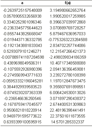
T = {a, ?}, the set of random constants R = {0, 1, 2, 3, 4, 5, 6, 7, 8, 9}, and the ephemeral random constant ‘?’ ranged over the interval [-1, 1]. The set of 20 random fitness cases chosen from the interval [-1,1]
is shown in Table 3 and the fitness was evaluated by a variant of equation
2.12 (Ferreira
2001):
|

|
(3.3) |
If  (the precision) less than or equal to 0.01%, then the precision is equal to zero and
f(i,j) = M. For this problem,
M = 100% and Ct = 20; therefore, fmax = 2000.
Table 3
Set of 20 random fitness cases used in the finding of the ‘V’ shaped function.

In this experiment, 100 identical runs were made. The parameters used per run are shown in the first column of
Table 4. The best solution was found in run 79 after 3619 generations.
Table 4
General settings used in the finding of the ‘V’ shaped function with and without random constants.
| |
With Random
Constants |
Without Random
Constants |
| Number
of runs |
100 |
100 |
| Number
of generations |
5000 |
5000 |
| Population
size |
100 |
100 |
| Number
of fitness cases |
20 (Table
3) |
20 (Table
3) |
| Function
set |
+
- * / L E K ~ S C |
+
- * / L E K ~ S C |
| Head
length |
6 |
6 |
| Number
of genes |
4 |
5 |
| Linking
function |
+ |
+ |
| Chromosome
length |
80 |
65 |
| Mutation
rate |
0.044 |
0.044 |
| One-point
recombination rate |
0.3 |
0.3 |
| Two-point
recombination rate |
0.3 |
0.3 |
| Gene
recombination rate |
0.1 |
0.1 |
| IS
transposition rate |
0.1 |
0.1 |
| IS
elements length |
1,2,3 |
1,2,3 |
| RIS
transposition rate |
0.1 |
0.1 |
| RIS
elements length |
1,2,3 |
1,2,3 |
| Gene
transposition rate |
0.1 |
0.1 |
| Rand.
const. mut. rate |
0.01 |
-- |
| Dc
specific IS transp. rate |
0.1 |
-- |
| Dc
specific IS elements length |
1,2,3 |
-- |
| Selection
range |
100% |
100% |
| Precision |
0.01% |
0.01% |
| Average
best-of-run fitness |
1850.476 |
1934.619 |
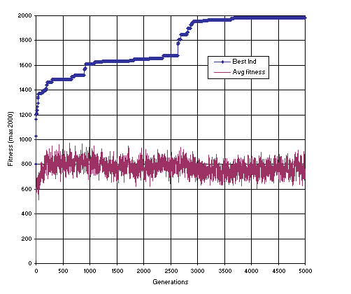
Figure 13 shows the progression of average fitness of the population and the fitness of the best individual for run 79 of this experiment.

Figure 13. Progression of average fitness of the population and the fitness of the best individual of run 79 of the experiment summarized in
Table 4, column 1 (function finding with random constants).
The best of run solution in terms of R-square is shown below (the sub-ETs are linked by addition):
|
Gene 0: L*~*+/aa?a??a2132990
A0 = {0.565, 0.203, 0.613, 0.219, 0.28, 0.25, 0.48, 0.427, 0.821, 0.127}
Gene 1: E-+-*?aaaaaaa7332660
A1 = {0.031, 0.046, 0.696, 0.643, 0.528, 0.417, 0.978, 0.811, 0.637, 0.988}
Gene 2: ~Saaa+??aa??a9109969
A2 = {0.515, 0.466, 0.254, 0.219, 0.425, 0.942, 0.306, 0.619, 0.821, 0.262}
Gene 3: ~SSaES?????aa5420661
|
|
|
A3 = {0.595, 0.547, 0.525, 0.219, 0.297, 0.387, 0.508, 0.695, 0.728, 0.415} |
(3.4) |
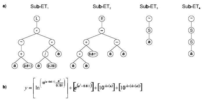
It has a fitness of 1975.264 and an R-square of 0.9999439 evaluated over the set of 20 fitness cases and an R-square of 0.9999075 evaluated against a test set of 100 random points. Its expression is shown in
Figure 14. This model is a very good approximation to the
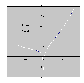
target function 3.2 as both the R-square and the comparison of the plots for the target function and the model show
(Figure 15).

Figure 14. Model 3.4 evolved by GEP using the facility for manipulation of random constants.
a) The sub-ETs codified by each gene. b) The
corresponding mathematical expression after linking with addition (the contribution of each sub-ET is shown in square brackets).

Figure 15. Comparison of the target function with the model
3.4 evolved by GEP using random constants (Figure
14). The R-square was evaluated over the test set of 100 random points and is equal to 0.9999075.
It is worth noticing that, despite integrating constants in the evolved solutions, the constants are very different from the expected ones. Indeed, GEP (and I believe, all genetic algorithms) can find the expected constants with a precision to the third or fourth decimal place when the target functions are simple polynomial functions with rational coefficients and/or when we could guess pretty accurately the function set, otherwise a very creative solution would be found. I don’t think this should be seen as a weakness of evolutionary algorithms for “constants” is apparently just another word for mathematical expression.
|


