The aim of this section is to study a successful run in its entirety in order to understand how populations of GEP individuals evolve towards a perfect or good solution.

In symbolic regression or function finding the goal is to find an expression that satisfactorily explains the dependent variable. The input into the system is a set of fitness cases in the form (a_(i,0), a_(i,1), ..., a_(i,n-1), y_i) where a_(i,0) - a_(i,n-1) are the independent variables and y_i is the dependent variable. The set of fitness cases consists of the adaptation environment where solutions adapt, discovering, in the process, solutions to problems.

In the example of this section, a simple test function was chosen, being therefore the fitness cases computer generated. Thus, in this case, we know exactly which function we are aiming at (remember, however, that in real-world problems the function is obviously unknown). So, suppose we are given a sampling of the numerical values from the curve:

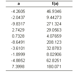
over 10 randomly chosen points in the real interval [-10, +10] and we wanted to find a function fitting those values within a certain error. In this case, we are given a sample of data in the form of 10 pairs (a_i, y_i), where a_i is the value of the independent variable in the given interval and y_i is the respective value of the dependent variable (Table 1). These 10 pairs are the fitness cases (the input) that will be used as the adaptation environment. The fitness of a particular program will depend on how well it performs in this environment.

Table 1
Set of 10 random fitness cases used in the simple problem of symbolic regression.

There are five major steps in preparing to use gene expression programming, and the first is to choose the fitness function. For this problem we could measure the fitness f_i of an individual program i by the following expression:

where M is the range of selection, C_(i,j) the value returned by the individual chromosome i for fitness case j (out of C_t fitness cases) and T_j is the target value for fitness case j. If |C_(i,j) - T_j| (the precision) less than or equal to 0.01, then the precision is equal to zero, and f_i = f_max = C_t*M. For this problem, we will use an M = 100 and, therefore, f_max = 1000. The advantage of this kind of fitness function is that the system can find the optimal solution for itself (Ferreira 2001).

The second major step consists in choosing the set of terminals T and the set of functions F to create the chromosomes. In this problem, the terminal set consists obviously of the independent variable, i.e., T = {a}. The choice of the appropriate function set is not so obvious, but a good guess can always be done in order to include all the necessary functions. In this case, to make things simple, we will use the four basic arithmetic operators. Thus, F = {+, -, *, /}.

The third major step is to choose the chromosomal architecture, i.e., the length of the head and the number of genes. In this problem we will use an h = 6 and three genes per chromosome.

The fourth major step in preparing to use gene expression programming is to choose the linking function. In this case we will link the sub-ETs by addition.

And finally, the fifth major step is to choose the set of genetic operators that cause variation and their rates. In this case we will use a combination of all genetic operators (mutation, the three kinds of transposition, and the three kinds of recombination) (see Table 2).

The parameters used per run are summarized in Table 2. I chose a small population of 20 individuals for this problem in order to simplify the analysis of the evolutionary process and not fill this text with pages of encoded individuals. However, one of the advantages of GEP is that it is capable of solving relatively complex problems using small population sizes and, thanks to the compact Karva notation, it is possible to fully analyze the evolutionary history of a run.

Table 2
Parameters for the simple symbolic regression problem.

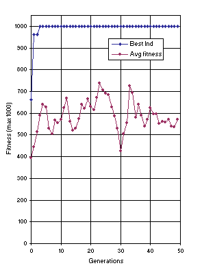
Figure 6 shows the progression of average fitness and the fitness of the best individual of a successful run. In this run, a perfect solution was found in generation 3.

Figure 6. Progression of average fitness of the population and the fitness of the best individual for a successful run of the experiment summarized in Table 2.

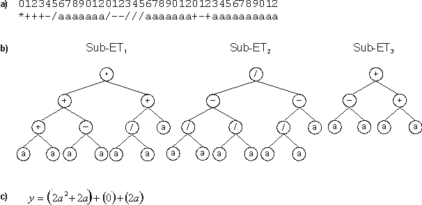
The initial population of this run, together with the fitness of each individual, is shown in Figure 7. Note that three of the 20 individuals are nonviable and thus have fitness zero. The best of generation individual, chromosome 19, has fitness 661.5933. Its expression and the corresponding mathematical equation are shown in Figure 8. Note that gene 2 returns zero and, therefore, might be considered a pseudogene. Note also how the algorithm created constants in all sub-ETs on its own.

Figure 7. Initial population (generation 0) for the simple problem of symbolic regression. For each problem, such an initial, totally random population is generated. The value after each chromosome indicates the fitness for the set of fitness cases shown in Table 1.

Figure 8. Best individual of generation 0 (chromosome 19 of Figure 7). It has a fitness of 661.5933. a) The chromosome of the individual. b) The sub-ETs codified by each gene. c) The corresponding mathematical expression after linking with addition (the contribution of each sub-ET is shown in brackets).

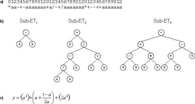
The descendants of the individuals of the initial population are shown in Figure 9. Note that chromosome 0 is the clone of the best individual of the previous generation. In this generation, a new individual was created, chromosome 7, considerably better than the best individual of the initial population. This chromosome has a fitness of 961.8512 and its expression is shown in Figure 10.

Figure 9. The descendants of the individuals of the initial population of Figure 7. The value after each chromosome indicates the fitness for the set of fitness cases shown in Table 1. Note that chromosome 0 is the clone of the best individual of the previous generation. In fact, this position is always occupied by the clone of the best individual of the previous generation.

Figure 10. Best individual of generation 1 (chromosome 7 of Figure 9) with a fitness of 961.8512. a) Its chromosome. b) The sub-ETs codified by each gene. c) The corresponding mathematical expression after linking with addition (the contribution of each sub-ET is shown in brackets).

The descendants of the individuals of this generation are shown in Figure 11 (generation 2). Note that despite the global improvement in fitness (compare the average fitness of both populations in Figure 6), none of the descendants surpassed the best individual of the previous generation.

Figure 11. The chromosomes of two populations for the simple problem of symbolic regression. The value after each chromosome indicates the fitness for the set of fitness cases shown in Table 1. In generation 2, none of the individuals surpassed the best of the previous generation. In generation 3, a perfect solution with maximum fitness was found (chromosome 13).

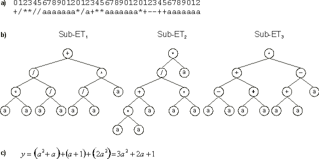
And finally, in the next generation (generation 3 of Figure 11), an individual with maximum fitness was created. Note that this chromosome is a descendant, via mutation, of chromosome 18 of the previous generation: their chromosomes differ only in one position (the ‘-’ at position 2 of gene 1 was replaced by ‘*’). The expression of this chromosome shows that it codes for a perfect solution (Figure 12).

Figure 12. Perfect solution found in generation 3 (chromosome 13 of Figure 11). It has the maximum value 1000 of fitness. a) The chromosome of this individual. b) The sub-ETs codified by each gene. c) The corresponding mathematical expression after linking with addition (the contribution of each sub-ET is shown in brackets).