To solve the sequence induction problem without the facility to manipulate numerical constants, the function set is exactly the same as in the experiment with random constants. The terminal set consists obviously of the independent variable alone.
As shown in the second column of Table
4.7, the probability of success using this approach is 98%, considerably higher than the 24% obtained using the facility to manipulate random constants. The first perfect solution, found in generation 89 of run 0, is shown below (the sub-ETs are linked by addition):
| 01234567890120123456789012012345678901201234567890120123456789012 |
|
|
**+++*aaaaaaa*+aaa-aaaaaaa-a*a/aaaaaaaa-**a/*aaaaaaa*--aaaaaaaaaa |
(4.16) |
As its expression shows, this program corresponds to the target
sequence. Note how the algorithm creates all the necessary constants from scratch by performing simple arithmetical operations.
To find the “V” shaped function without the facility for the manipulation of random constants, the function set is exactly the same as in the first approach. With this collection of functions, most of which extraneous, the algorithm is equipped with different tools for evolving highly accurate models without explicitly using numerical constants. The parameters used per run are shown in the second column of
Table 4.9.
The best solution of this experiment was found in generation 2790 of run 39 (the sub-ETs are linked by addition):
| 01234567890120123456789012012345678901201234567890120123456789012 |
|
|
+L+*a~aaaaaaa*aCK+/aaaaaaa*S*C~Caaaaaaa*~CEC-aaaaaaaS*SC+/aaaaaaa |
(4.17a) |
It has a fitness of 1991.887 and an R-square of 0.99992182 evaluated over the set of 20 fitness cases and an R-square of 0.9998882 evaluated against the same testing set used in the first approach, and thus is better than the model
(4.12) evolved with the facility to manipulate random constants. More formally, the model
(4.17a) can be expressed by the following C++ function:
double APSCfunction(double d[ ])
{
double
dblTemp = 0;
dblTemp
+= (log((d[0]*d[0]))+(d[0]+pow(10,d[0])));
dblTemp
+= (d[0]*cos(log10(((d[0]/d[0])+d[0]))));
dblTemp
+= (sin(cos(d[0]))*(pow(10,d[0])*cos(d[0])));
dblTemp
+= (pow(10,exp((d[0]-d[0])))*cos(cos(d[0])));
dblTemp
+= sin((sin((d[0]+d[0]))*cos((d[0]/d[0]))));
return
dblTemp; |
|
|
} |
(4.17b) |
where d0 corresponds to the independent variable
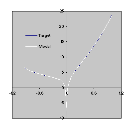
a. Once again, the plots of the target function and the model evolved by GEP are compared in
Figure 4.8.

Figure 4.8. Comparison of the target function (4.10) with the model
(4.17) evolved by GEP without explicitly using random constants. The R-square was evaluated over a testing set of 100 random points and is equal to 0.9998882.
For predicting sunspots without explicitly using random constants, the function set was exactly the same as in the first approach. The parameters used per run are shown in the second column of
Table 4.10. The best solution of this experiment was found in generation 2284 of run 45 (the sub-ETs are linked by addition):
| 012345678901234012345678901234012345678901234 |
|
|
//+*-dehjiecfceji--ac/efbhjcjf/*+-ji+biaifgdf |
(4.18a) |
It has a fitness of 89184.62 and an R-square of 0.884351 evaluated over the set of 90 fitness cases and, thus, is better than the model
(4.13) evolved with the facility to manipulate random constants. More formally, the model
(4.18a) can be expressed by the following function:
|

|
(4.18b) |
It is instructive to compare the results obtained with both approaches. In all the experiments, the explicit use of random constants resulted in considerably worse performance. In the sequence induction problem, the success rate is much higher if the algorithm created the numerical constants from scratch; specifically, success rates of 98% against 24% were obtained (see
Table 4.7). In the “V” function problem, the average best-of-run fitness is also considerably higher when the algorithm was allowed to invent new ways of representing numerical constants; in this case, average best-of-run fitnesses of 1953.057 against 1896.25 and average best-of-run R-squares of 0.99647004 against 0.95129456 were obtained (see
Table 4.9). And in the sunspots prediction task, average best-of-run fitnesses of 89009.66 against 86182.05 and average best-of-run R-squares of 0.801144 against 0.706437 were obtained (see
Table 4.10). Thus, in real-world applications where complex realities are modeled, of which neither the type nor the range of the numerical constants are known, and where most of the times it is impossible to guess the exact function set, it is more appropriate to let the system model the reality on its own, that is, with a toolkit devoid of random constants. Not only the results will be better but also the complexity of the system will be much smaller. And the simpler the system the faster evolution.
In the next section, though, we are going to analyze a kind of problem where random constants are absolutely necessary.
|
