To solve the sequence induction problem using the facility to manipulate random constants, the set of functions
F = {+, -, *} and the set of terminals T = {a, ?}. Furthermore, a set of integer random constants represented by the numerals 0-9 was used, that is,
R = {0, 1, 2, 3, 4, 5, 6, 7, 8, 9}. The ephemeral random constant “?” ranged over the integers 0, 1, 2, and 3. The parameters used per run are shown in the first column of
Table 4.7.
The perfect solution shown below was discovered on generation 99 of run 0 (the sub-ETs are linked by addition):
|
Gene 0: ***a+*aaaa?a?4044044
A0 =
{0, 1, 3, 0, 2, 0, 1, 1, 0, 1}
Gene 1: **+*a?a?aa???3858227
A1 =
{3, 2, 2, 1, 3, 1, 1, 0, 3, 2}
Gene 2: /?a-?-a????aa5011303
A2 =
{3, 2, 0, 0, 1, 0, 2, 1, 3, 1}
Gene 3: -?-*-aa??a?aa5485938
A3 =
{3, 0, 1, 2, 0, 3, 3, 1, 3, 3}
Gene 4: a**/*aaa?aaaa2416267
|
|
|
A4 = {0, 2, 0, 2, 2, 2, 1, 0,
3, 3} |
(4.11) |
As its expression shows, this program matches exactly the target sequence
(4.9).
As shown in Table 4.7, the probability of success for this problem is 24%, considerably lower than the 98% obtained using the second approach. Surprisingly, the inclusion of numerical constants in the evolutionary toolkit results in worse performance. Thus, evolutionary algorithms find the numerical constants more easily if no assumptions whatsoever are a priori made. It is worth pointing out that only the prior knowledge of the solution enabled us, in this case, to choose correctly the type and the range of the random constants.
To find the “V” shaped function by explicitly using random constants
F = {+, -, *, /, L, E, K, ~, S, C} (“L” represents the natural logarithm, “E” represents
ex, “K” represents the logarithm of base 10, “~” represents
10x, “S” represents the sine function, and “C” represents the cosine) and
T = {a, ?}. The set of rational random constants R = {0, 1, 2, 3, 4, 5, 6, 7, 8, 9}, and “?” ranged over the interval [-1, 1]. The parameters used per run are shown in the first column of
Table 4.9. In the best run of this experiment, the best solution was found in generation 3631. Its genome is shown below (the sub-ETs are linked by addition):
|
Gene 0: ++?~a*a???a?a0643987
A0 =
{0.03, 0.019, 0.419, 0.247, 0.367, 0.689, 0.648, 0.245, 0.252,
0.904}
Gene 1: ~S/aSE?a?aaaa5670520
A1 =
{0.476, 0.477, 0.786, 0.196, 0.92, 0.344, 0.934, 0.198, 0.107,
0.575}
Gene 2: ~CCLE*aa?a??a1654524
A2 =
{0.298, 0.083, 0.466, 0.404, 0.912, 0.782, 0.392, 0.223,
0.548, 0.43}
Gene 3: /LE/-*?aaaaa?4324454
A3 =
{0.947, 0.357, 0.549, 0.338, 0.465, 0.435, 0.837, 0.776,
0.602, 0.593}
Gene 4: ~*aCaE???aaa?8125208
|
|
|
A4 = {0.189, 0.357, 0.494,
0.38, 0.465, 0.88, 0.995, 0.971, 0.966, 0.294} |
(4.12a) |
It has a fitness of 1978.177 and an R-square of 0.999914 evaluated over the set of 20 fitness cases and an R-square of 0.999216 evaluated against a testing set of 100 random points also chosen from the interval [-1, 1]. More formally, it corresponds to the following C++ function:
double APSCfunction(double d[ ])
{
double
dblTemp = 0;
dblTemp
+= ((pow(10,(d[0]*0.648))+d[0])+0.03);
dblTemp
+= pow(10,sin((d[0]/sin(exp(0.344)))));
dblTemp
+= pow(10,cos(cos(log(exp((d[0]*d[0]))))));
dblTemp
+= (log(((d[0]*d[0])/0.465))/exp((d[0]-d[0])));
dblTemp
+= pow(10,(d[0]*cos(d[0])));
return
dblTemp; |
|
|
} |
(4.12b) |
where d0 corresponds to the independent variable.
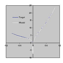
This model is a very good approximation to the target function (4.10) as both the R-square and the comparison of the plots for the target function and the model show
(Figure 4.7).

Figure 4.7. Comparison of the target function (4.10) with the model
(4.12) evolved by GEP with the facility to manipulate random constants. The R-square was evaluated over a testing set of 100 random points and is equal to 0.999216.
And, finally, for predicting sunspots using the facility for the manipulation of random numerical constants
F = {+, -, *, /} and T = {a, b, c,
d, e, f, g, h, i, j, ?}, which correspond, respectively, to
t-10, t-9, ..., t-1. The set of rational random constants
R = {0, 1, 2, 3, 4, 5, 6, 7, 8, 9}, and “?” ranged over the interval [-1, 1]. The parameters used per run are shown in the first column of
Table 4.10. The best solution, found in run 90 after 4945 generations, is shown below (the sub-ETs are linked by addition):
|
Gene 0: /*+i*h+?hfddh?c29898626
A0 =
{0.387, 0.375, 0.373, 0.606, 0.363, 0.958, 0.211, 0.062, 0.12,
0.239}
Gene 1: *j/j++ii?afc?ad03960507
A1 =
{0.274, 0.472, 0.153, 0.38, 0.887, 0.828, 0.378, 0.779, 0.414,
0.065}
Gene 2: /+++a++agee?gjd89794029
|
|
|
A2 = {0.433, 0.503, 0.333, 0.092, 0.066, 0.245, 0.592, 0.43, 0.051,
0.998} |
(4.13a) |
It has a fitness of 86733.21 and an R-square of 0.84312712 evaluated over the set of 90 fitness cases. Mathematically, it corresponds to the following function:
|

|
(4.13b) |
It is worth noticing that, using this approach, the algorithm does in fact integrate constants in the evolved solutions, but the constants are, at least in some cases, very different from the expected ones (compare, for instance, the model of the “V” function with the function itself). Indeed, gene expression programming (and I believe, all evolutionary algorithms) can find the expected constants with a precision to the third or fourth decimal place if the target functions are simple polynomial functions with rational coefficients, otherwise a very creative solution will be found. For instance, the simple function below:
|
y = 2.718a2
+ 3.1416a |
(4.14) |
can be exactly solved by GEP using the facility to manipulate random constants (see the performance and parameters in
Table 4.11).
Table 4.11
Settings for the polynomial function with rational coefficients.
| Number
of runs |
100 |
| Number
of generations |
1000 |
| Population
size |
50 |
| Number
of fitness cases |
10 (Table
4.12) |
| Function
set |
+
- * / |
| Terminal
set |
a ? |
| Random
constants array length |
10 |
| Random
constants range |
[-1,1] |
| Head
length |
6 |
| Number
of genes |
2 |
| Linking
function |
+ |
| Chromosome
length |
40 |
| Mutation
rate |
0.044 |
| One-point
recombination rate |
0.3 |
| Two-point
recombination rate |
0.3 |
| Gene
recombination rate |
0.1 |
| IS
transposition rate |
0.1 |
| IS
elements length |
1,2,3 |
| RIS
transposition rate |
0.1 |
| RIS
elements length |
1,2,3 |
| Gene
transposition rate |
0.1 |
| Random
constants mutation rate |
0.01 |
| Dc
specific transposition rate |
0.1 |
| Dc
specific IS elements length |
1,2,3 |
| Selection
range |
25% |
| Precision |
0% |
| Average
best-of-run fitness |
243.994 |
| Average
best-of-run R-square |
0.999826 |
Table 4.12
Set of fitness cases for the polynomial function.
| a |
f(a) |
| -8.5013 |
169.7278883 |
| -0.8696 |
-0.676572453 |
| 3.7181 |
49.25514232 |
| 5.0878 |
86.34118911 |
| -4.313 |
37.01043094 |
| 1.9775 |
16.84126999 |
| -8.767 |
181.3638583 |
| -5.5617 |
66.60191701 |
| -1.4234 |
1.035098188 |
| 6.9014 |
151.1379353 |
Consider, for instance, the almost perfect solution below:
|
Gene 0: *+++*+?aaa?a?4673929
A0 =
{0.244, 0.966, 0.461, 0.762, 0.409, 0.567, 0.718, 0.746, 0.993,
0.236}
Gene 1: **??aa???a??a8610121
|
|
|
A1 = {0.103, 0.086, 0.038, 0.793, 0.307, 0.062, 0.051, 0.025, 0.046,
0.911} |
(4.15a) |
It has an R-square equal to 0.999999999769 and, therefore, is an almost perfect match to the
target function. Indeed, as its mathematical expression shows, the algorithm discovered the numerical constants of equation
(4.14) with great precision:
|
y = 2.718a2
+ 3.14163a |
(4.15b) |
|
