The target function of this section is the simple polynomial:
|
y = a3 +
a2 + a + 1 |
(4.1) |
This function was chosen not only because it allows the execution of hundreds of runs in a few seconds but also because it can be solved exactly by the algorithm. Consequently, it can be used to illustrate how to choose the appropriate settings for a problem, including the fitness function, the number of genes, the head length, the function set and the linking function. This kind of analysis is useful for developing an intuitive understanding of the fundamental parameters of the algorithm. The parameters chosen for this problem are summarized in
Table 4.1; how and why they were chosen is discussed below.
Table 4.1
Settings for the polynomial function problem.
| Number
of runs |
100 |
| Number
of generations |
50 |
| Population
size |
30 |
| Number
of fitness cases |
10 (Table
4.2) |
| Function
set |
+
- * / |
| Terminal
set |
a |
| Head
length |
6 |
| Number
of genes |
4 |
| Linking
function |
+ |
| Chromosome
length |
52 |
| Mutation
rate |
0.0385 |
| One-point
recombination rate |
0.3 |
| Two-point
recombination rate |
0.3 |
| Gene
recombination rate |
0.1 |
| IS
transposition rate |
0.1 |
| IS
elements length |
1,2,3 |
| RIS
transposition rate |
0.1 |
| RIS
elements length |
1,2,3 |
| Gene
transposition rate |
0.1 |
| Selection
range |
100% |
| Precision |
0.01% |
| Success
rate |
100% |
Consider we are given a sampling of the numerical values from the test function
(4.1) over 10 random points chosen from the interval [-10, 10], and we wanted to find a function fitting those values within 0.01 of the correct value.
First, the set of functions and the set of terminals must be chosen. In this case we could choose
F = {+, -, *, /} and T = {a}. Next, the structural organization of chromosomes, namely, the length of the head
h and the number of genes, must also be chosen. It is wise to start with short, single-gene chromosomes and then gradually increase
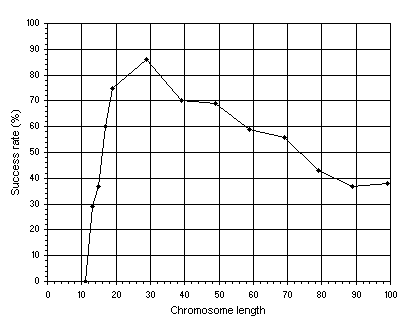
h. Figure 4.1 shows such an analysis for this problem. Note how the success rate increases abruptly in the beginning, from a small success rate of 29% for the most compact organization (a gene length
g of 13) to a high success rate of 86% obtained with a moderately redundant organization
(g = 29). Note also that, from this point onward, the success rate starts to decrease progressively. As you can see, for each search landscape it is possible to guess more or less accurately the ideal chromosome length so that the landscape is thoroughly explored.

Figure 4.1. Variation of success rate with chromosome length. For this analysis, chromosomes composed of one gene were used,
G = 50, and P = 30. The success rate was evaluated over 100 identical runs.
As shown in Table 4.1, for this analysis, a population size
P of 30 individuals and an evolutionary time G of 50 generations were used. In all the experiments, only mutation and two-point recombination were used in order to simplify the analysis. The mutation rate was equivalent to two one-point mutations per chromosome and the recombination rate was equal to 0.7. The set of 10 random fitness cases used in this problem was chosen from the interval [-10, 10]
(Table 4.2). The fitness was evaluated by equation
(3.1a); in this case, a selection range of 100 and a precision of 0.01 were chosen. Thus, for a set of 10 fitness cases,
fmax = 1000.
Table 4.2
Set of fitness cases used in the polynomial function problem.
| a |
f(a) |
| 5.7695 |
232.107 |
| -4.1206 |
-56.1063 |
| 4.652 |
127.968 |
| -5.6193 |
-150.481 |
| -3.2971 |
-27.2686 |
| -0.0599 |
0.943473 |
| 1.1835 |
5.24187 |
| -8.2814 |
-506.651 |
| 4.4342 |
112.282 |
| 4.1843 |
95.9529 |
Note that GEP can be used to search the most parsimonious solution to a problem. As shown in
Figure 4.1, it was not possible to find a correct solution to this problem using a head length of five. Only with
h = 6 was it possible to evolve a perfect solution. In this case, these perfect solutions are also the most parsimonious solutions to the problem at hand. For instance, the following chromosomes:
|
0123456789012
*++/*/aaaaaaa-[1]
*++*//aaaaaaa-[2] |
both code for perfect, parsimonious solutions each with 13 nodes.
Note also that GEP can evolve solutions efficiently using large values of
h, i.e., is capable of dealing with uncompressed and highly redundant information. As shown in
Figure 4.1, for each problem, there is a chromosome length that allows the most efficient evolution. And, at least for simple test problems, this ideal chromosome length can be easily found. Note also that the most compact genomes are not the most efficient. This suggests that a certain redundancy is fundamental to the efficient evolution of good programs (see
chapter 7 for a discussion).
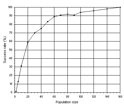
In the next experiment we are going to analyze the relationship between success rate and population size
P (Figure 4.2). Note that a medium value for the head
(h = 19) was used in order to have some resolution in the plots. Indeed, not only the
h chosen was not the most advantageous (see Figure
4.1), but also single-gene chromosomes were used. Remember, though, that GEP is much more complex than a unigenic system as GEP chromosomes can code for multiple genes.

Figure 4.2. Variation of success rate with population size in unigenic systems. For this analysis
G = 50 and a medium value of 39 for chromosome length
(h = 19) was used. The success rate was evaluated over 100 identical runs.
Suppose that, after the analysis shown in Figures 4.1 and
4.2, we could not find a satisfactory solution or the system was not evolving efficiently. Then we could choose a multigenic system and obviously choose how to link the expression trees. For instance, we could choose genes with an
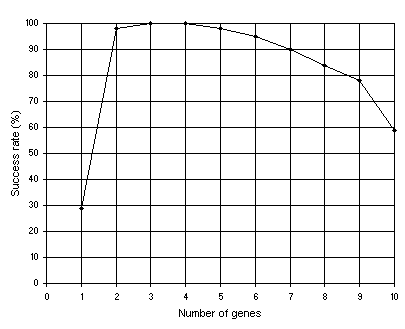
h = 6 encoding sub-ETs linked by addition. Figure 4.3 shows such an analysis for this problem. In this experiment, the mutation rate was equivalent to two one-point mutations per chromosome and, therefore, varies according to chromosome length,
p1r = p2r = 0.3, pgr
= pgt = pis = pris
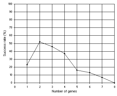
= 0.1, and three transposons (both IS and RIS elements) of lengths 1, 2, and 3 were used. Note that gene expression programming can cope very well with an excess of genes: the success rate for the 10-genic system is still very high (59%). Again we can see that a certain amount of redundancy allows a greater efficiency. In this case, chromosomes encoding between two and six sub-ETs linked by addition are extremely successful in the exploration of this particular solution landscape.

Figure 4.3. Variation of success rate with the number of genes. For this analysis
G = 50, P = 30, h = 6 (a gene length of 13), and the sub-ETs were linked by addition. The success rate was evaluated over 100 identical runs.
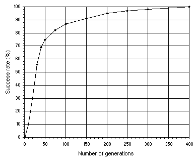
In Figure 4.4 another important relationship is shown: how the success rate depends on the number of generations
G. For this analysis, single-gene chromosomes with a relatively high chromosome length
g = 79 (h = 39) were used so that we could have resolution at high values of
G. The general parameters used in this analysis are exactly the same as in the analysis shown in
Figure 4.1. As Figure 4.4
emphasizes, in GEP, populations can adapt and evolve indefinitely because new material is constantly being introduced in the genetic pool.

Figure 4.4. Variation of success rate with the number of generations. For this analysis
P = 30 and a chromosome length of 79 (a single-gene chromosome with
h = 39) was used. The success rate was evaluated over 100 identical runs.
Finally, suppose that the multigenic system with sub-ETs linked by addition could not evolve a satisfactory solution to the problem at hand. Then we could choose another linking function or let the system evolve the linking functions on its own. In the analysis shown in
Figure 4.5, multiplication was used as linking function. The remaining parameters are exactly the same as in the analysis shown in
Figure 4.3.

Figure 4.5. Variation of success rate with the number of genes. For this analysis
G = 50, P = 30, h = 6 (a gene length of 13), and the sub-ETs were linked by multiplication. The success rate was evaluated over 100 identical runs.
As expected, for this polynomial function, the algorithm excelled with multigenic chromosomes encoding sub-ETs posttranslationally linked by addition. This testing of waters is done until a good solution has been found or a feel for the best chromosomal structure and composition is developed. Then, one selects the appropriate settings and lets the system evolve the best possible solution on its own.
Consider, for instance, the multigenic system composed of four genes linked by addition. As shown in
Figure 4.3, the success rate has, in this case, the maximum value of 100%, meaning that, in all the runs, a perfect solution was found. Let us analyze with more detail a successful run of this experiment. The parameters used per run are summarized in
Table 4.1 above.
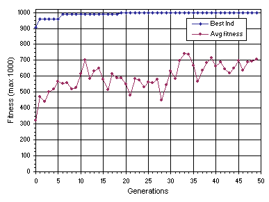
The evolutionary dynamics of this successful run (run 0) is shown in
Figure 4.6. As you can see, a perfect solution was found in generation 19.

Figure 4.6. Progression of average fitness of the population and the fitness of the best individual for run 0 of the experiment summarized in
Table 4.1.
The chromosomes and fitnesses of the individuals of the initial population of this run are shown below (the best individual of this generation is shown in
blue):
|
Generation N: 0
0123456789012012345678901201234567890120123456789012
**//++aaaaaaa/a//**aaaaaaa++/-**aaaaaaa+/+-aaaaaaaaa-[ 0] = 479.9631
*/-//+aaaaaaa/*+a/aaaaaaaa--aa//aaaaaaa-+/++*aaaaaaa-[ 1] = 354.6601
-+a/a/aaaaaaa/-/+-*aaaaaaa*-*/+/aaaaaaa*/a-/aaaaaaaa-[ 2] = 373.0389
---//+aaaaaaa*+/a--aaaaaaa++aa+aaaaaaaa**+++-aaaaaaa-[ 3] = 193.9366
/--aa/aaaaaaa+-a+--aaaaaaa//+a/-aaaaaaa-/+a*+aaaaaaa-[ 4] = 287.6966
-*/a/+aaaaaaa*+/+-/aaaaaaa/-*++*aaaaaaa+++-a/aaaaaaa-[ 5] = 355.6841
*aaaa*aaaaaaa*a-/-*aaaaaaa/--*+/aaaaaaa++*-*aaaaaaaa-[ 6] = 408.3963
--/++aaaaaaaa*a//++aaaaaaa///a-aaaaaaaa*+a++*aaaaaaa-[ 7] = 0
---**aaaaaaaa*-++++aaaaaaa*/aa+aaaaaaaa--aa/aaaaaaaa-[ 8] = 319.8496
/-/+--aaaaaaa+---/*aaaaaaa*--*-+aaaaaaa/*aa+*aaaaaaa-[ 9] = 0
-**/-+aaaaaaa*+aa-/aaaaaaa-/-a*+aaaaaaa*+-+++aaaaaaa-[10] = 324.3444
+a/-/-aaaaaaa-+*/+-aaaaaaa/-/a/-aaaaaaa+-++-aaaaaaaa-[11] = 0
+a+*--aaaaaaa-+-*+-aaaaaaa+a///-aaaaaaa+//a+-aaaaaaa-[12] = 412.0092
/a/-/-aaaaaaa*+/*-*aaaaaaa**a/*+aaaaaaa*--+aaaaaaaaa-[13] = 215.5287
***/*/aaaaaaa-*//-aaaaaaaa//-a-aaaaaaaa/*/-+-aaaaaaa-[14] = 0
-a+/a+aaaaaaa--*a/+aaaaaaa-**-+aaaaaaaa-/+++/aaaaaaa-[15] = 420.3384
//+a-*aaaaaaa/a-a*+aaaaaaa**+/-aaaaaaaa/+-a/-aaaaaaa-[16] = 0
+-aa/+aaaaaaa-*-**aaaaaaaa*//*-/aaaaaaa*+*a/aaaaaaaa-[17] = 0
*/-+a*aaaaaaa+*-+-/aaaaaaa/a-//aaaaaaaa-+-/+aaaaaaaa-[18] = 0
+-++a-aaaaaaa+-a*-aaaaaaaa/*a---aaaaaaa+*a+a*aaaaaaa-[19] = 789.56
+*aa++aaaaaaa*++a+/aaaaaaa+*/**/aaaaaaa*/*/*-aaaaaaa-[20] = 171.441
/a**a/aaaaaaa*+-++/aaaaaaa*//-++aaaaaaa----/-aaaaaaa-[21] = 403.2058
+a*--aaaaaaaa+/-//-aaaaaaa--++a*aaaaaaa+***aaaaaaaaa-[22] = 779.5309
*////*aaaaaaa-//-a/aaaaaaa/*/a-+aaaaaaa+-/*+*aaaaaaa-[23] = 296.2591
/a-++-aaaaaaa+-**a*aaaaaaa*+-a*aaaaaaaa-/+aa-aaaaaaa-[24] = 873.554
*a++/aaaaaaaa/-a--*aaaaaaa***a+/aaaaaaa*/*+a-aaaaaaa-[25] = 313.3738
-++/+/aaaaaaa*+a+*/aaaaaaa/+-+-/aaaaaaa-+//a+aaaaaaa-[26] = 908.0693
*/***/aaaaaaa+-*---aaaaaaa/+a/a*aaaaaaa*+*+/*aaaaaaa-[27] = 195.4805
+*a+/aaaaaaaa**a+-*aaaaaaa/*+a+/aaaaaaa+***a-aaaaaaa-[28] = 748.5801
-/---+aaaaaaa//+*+-aaaaaaa-/---aaaaaaaa+-++*-aaaaaaa-[29] = 0
|
Note that eight of the 30 randomly generated individuals are nonviable, that is, have zero fitness. This means that, either they were unable to solve a single fitness case within the chosen selection range, or they returned mathematical errors such as a division by zero. The best individual of this generation, chromosome 26, has fitness 908.0693. As its expression shows, two of the four terms of the
target function (the first and second terms) are already present in this solution.
In the next generation a new individual with better traits than the best individual of generation 0 was created:
|
0123456789012012345678901201234567890120123456789012 |
|
|
+a+*-aaaaaaaa+/-//-aaaaaaa--++a*aaaaaaa+***aaaaaaaaa |
(4.2) |
It has a fitness of 958.3982 evaluated against the set of fitness cases presented in
Table 4.2. Its expression shows that three of the terms of this intermediate solution match exactly the
target function; in fact, only the third term is missing.
As you can see in Figure 4.6, for the next four generations no improvement in best fitness was observed. But in generation 6 a better solution with fitness 990 was found:
|
0123456789012012345678901201234567890120123456789012 |
|
|
+-/-a-aaaaaaa+-a**aaaaaaaa*+-a*aaaaaaaa+*a+a*aaaaaaa |
(4.3) |
As its expression shows, three of the terms of this intermediate solution match exactly the
target function; in this case, only the last term is missing.
For the next 12 generations no improvement in best fitness occurred (see
Figure 4.6). But in generation 19 a perfect solution with maximum fitness was found:
|
0123456789012012345678901201234567890120123456789012 |
|
|
+*a/-aaaaaaaa*-/++aaaaaaaa-/***-aaaaaaa+***/*aaaaaaa |
(4.4) |
As its expression shows, it matches exactly the target function (4.1).
The detailed analysis of these best-of-generation programs shows that some of the actions are redundant or neutral, like the addition of zero or the multiplication by one. However, the existence of these redundant clusters, be they small neutral clusters in the sub-ETs or entire neutral genes like gene 2 in chromosome
(4.4) above, is important to the evolution of fitter individuals (compare, in Figures
4.1 and 4.3, the success rate of a compact,
unigenic system with
h = 6 with other less compact systems, either with more genes or head lengths greater than six).
Obviously, in real-world problems such an exhaustive analysis is impractical. For those problems one usually experiments with a couple of chromosomal organizations and tests different function sets. By observing such indicators as best and average fitness, it is easy to see whether the system is evolving efficiently or not. Then the appropriate settings are chosen and the system is left to evolve the best possible solution to the problem at hand.
|
