In this section we are going to use gene expression programming to design a computer program that can be used to diagnose breast cancer. The data sets used both for training and testing were obtained from PROBEN1 – a set of neural network benchmark problems and benchmarking rules (Prechelt 1994). Both the technical report and the data sets are available through anonymous FTP from Neural Bench archive at Carnegie Mellon University (machine ftp.cs.cmu.edu, directory /afs/cs/project/connect/bench/contrib/prechelt) and from the machine ftp.ira.uka.de in directory /pub/neuron. The file name in both cases is proben1.tar.gz.

In this diagnosis task the goal is to classify a tumor as either benign (0) or malignant (1) based on nine different cell analysis (input attributes or terminals).

The model presented here was obtained using the cancer1 data set of PROBEN1 where the binary 1-of-m encoding in which each bit represents one of m-possible output classes was replaced by a 1-bit encoding (“0” for benign and “1” for malignant). The first 350 samples were used for training and the last 174 samples were used to test the performance of the model in real use. This means that absolutely no information from the test set samples or the test set performance are available during the adaptive process. Thus, both the classification accuracy and classification error on the test set can be used to evaluate the generalization performance of the evolved models.

For this problem a very simple function set was chosen, composed only of the four arithmetic operators, that is, F = {+, -, *, /}, where each function was weighted five times; the set of terminals consisted of the nine attributes used in this problem and were represented by T = {d₀, ..., d₈} which correspond, respectively, to clump thickness, uniformity of cell size, uniformity of cell shape, marginal adhesion, single epithelial cell size, bare nuclei, bland chromatin, normal nucleoli, and mitoses.

In classification problems where the output is often binary, it is important to set criteria to convert real-valued numbers into zero or one. This is the 0/1 rounding threshold R_t that converts the output of a chromosome into “1” if the output is equal to or greater than R_t, or into “0” otherwise. For this problem we are going to use R_t = 0.1.

The fitness function used to evaluate the performance of each candidate model is very simple and is based on the number of samples correctly classified. Thus, the fitness f_i of an individual program corresponds to the number of hits and is evaluated by the formula:

where n is the number of sample cases correctly evaluated, and C_p is the number of samples in the class with more members (predominant class).

As it is customary in genetic programming (Koza 1992) and gene expression programming (Ferreira 2001), the parameters used per run are summarized in a table (Table 1). Note that, in this case, a small population of 50 individuals and chromosomes composed of three genes with an h = 8 and sub-ETs linked by addition were used. The program below was discovered after 423 generations (genes are shown separately and a dot is used to separate each element):

It has a fitness of 340 evaluated against the training set of 350 fitness cases and maximum fitness on the test set of 174 samples. This means that this model is very good indeed, with a classification accuracy of 100% and a classification error of 0% in the test set. In the training set a classification accuracy of 97.14% and a classification error of 2.86% were obtained.


Table 1
Settings used in the breast cancer problem.

Note that for the expression of chromosome (11a) to be complete the sub-ETs must be linked by addition and the 0/1 rounding threshold must be taken into account. With the software APS 3.0 by Gepsoft, the model (11a) above can be automatically converted into a fully expressed computer program or function, such as the C++ function below:

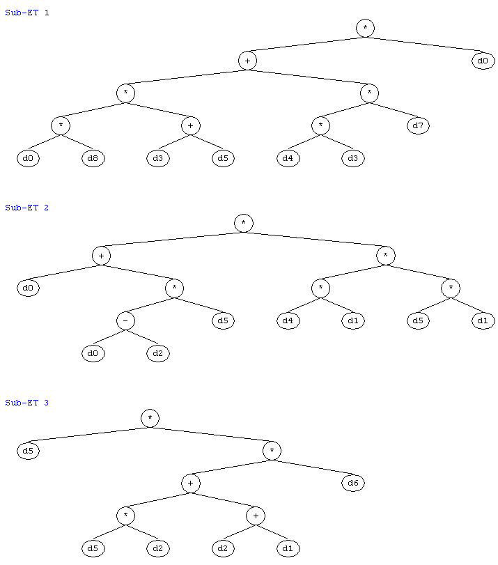
Similarly, all models evolved by gene expression programming can be immediately converted into virtually any programming language through the use of grammars, including the universal representation of parse trees (Figure 7). These trees can then be used to grasp immediately the mathematical intricacies of the evolved models and therefore are ideal for extracting knowledge from data.

Figure 7. The sub-ETs of the model (11b) evolved by gene expression programming to diagnose breast cancer. (Expression trees drawn by Gepsoft APS 3.0.)

As you can clearly see in Figure 7, all the cell analysis seem to be relevant to an accurate diagnosis of breast cancer. This is, indeed, one of the great advantages of gene expression programming: the possibility of extracting knowledge almost instantaneously as the models evolved by GEP can be represented in any conceivable language, including the universal diagram representation of expression trees.