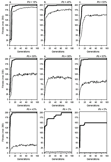
Figure 7.2. The dynamics of mutation. The success rate above each plot was determined in the experiment shown in Figure 7.1. a) Moderately Innovative (p_m = 0.001). b) Healthy But Weak (p_m = 0.0045). c) Healthy And Strong (p_m = 0.016). d) Healthy And Strong (p_m = 0.022). e) Healthy And Strong (p_m = 0.034). f) Unhealthy But Strong (p_m = 0.046). g) Unhealthy And Weak (p_m = 0.15). h) Almost Random (p_m = 0.45). i) Totally Random (p_m = 1.0). Note that, except for the last dynamics, only successful runs were chosen so that the plot for best fitness reached its maximum value and the distance between average and best fitness could be better appreciated.

In the first evolutionary dynamics, p_m = 0.001 and P_s = 16% (plot a), the plot for average fitness closely accompanies the plot for best fitness and only a small oscillation is observed in average fitness. These populations are called moderately innovative as they evolve very sluggishly and only a little bit of genetic diversity is introduced in the population.

In the second dynamics, p_m = 0.0045 and P_s = 48% (plot b), it can be observed that, although closely accompanying the plot for best fitness, the gap between both plots increases and the characteristic oscillatory pattern on average fitness is already evident even for such small variation rates. As shown in Figure 7.1, this population is midway to the peak with a success rate of 48%. Such systems, although adaptively healthy, are not very efficient and are called healthy but weak.

As shown in Figure 7.1, the success rate increases abruptly with mutation rate until it reaches a plateau around p_m = 0.022. In terms of dynamics, this is reflected in a more pronounced oscillatory pattern in average fitness and an increase in the gap between average and best fitness. For obvious reasons, populations evolving with maximum performance are called healthy and strong. The next three dynamics (plots c, d, and e) are all drawn from the performance plateau or peak. Note, however, that from the peak onward, an increase in mutation rate results in a decrease in performance until populations are totally incapable of adaptation (see Figure 7.1). In these populations, the gap between average and best fitness continues to increase (see plots f through i) until the plot for average fitness reaches the bottom and populations become totally random and incapable of adaptation (see plot i). Note also that some populations, despite evolving under excessive mutation, are still very efficient. For instance, the evolutionary dynamics shown in plot f, p_m = 0.046 and P_s = 93%, is extremely efficient. This kind of population is called unhealthy but strong (with “unhealthy” indicating the excessive mutation rate). The next population, p_m = 0.15 and P_s = 43% (plot g), is not as efficient as the previous one and therefore is called unhealthy and weak.

The last two dynamics were obtained for populations outside the finger region of the mutation plot. In the first, p_m = 0.45 and P_s = 3% (plot h), the plot for average fitness is not far from the minimum position obtained for totally random populations (plot i). Thus, populations of this kind are called, respectively, almost random and totally random. Note that oscillations on average fitness are less pronounced in these plots. It is worth noticing that totally random populations (the presence of elitism at p_m = 1.0 is, in this experiment with 500 individuals, insignificant in terms of average fitness) are unable to find a perfect solution to the problem at hand. And this tells us that every time a perfect solution was found, a powerful search mechanism was responsible for this and not a random search.